The Past
This section outlines our research into the past work completed in this space - in other words, our literature review. Significant work has been accomplished towards using satellite imagery for predicting yields of crops, and several models exist with varying spohistication from the USDA and other vendors. Our approach attempts to extend the existing body of work by predicting soybean yields in Brazil, incorporating weather data in addition to data from satellites.
This project uses vegetation indices calculated from MODIS satellite images to predict crop yields on a farm-by-farm basis 2. Our efforts abstract from the complicated mixture of factors that affect yields on the ground, such as soil conditions, pest pressures, weather, irrigation, fertilizer use, crop rotation, and other advanced farming methods. We assume that vegetation indices can capture the effects of all such surface inputs and that by applying the latest machine learning techniques, we can find patterns in the data that predict yields as accurately as more data-intensive models.
Several researchers, notably William Allen, Harold Gausman, and Joseph Woolley, have established how the optical properties of plants relate to their growth and productivity. The different wavelengths of light reflected by plants and soils create unique spectral signatures that indicate water content, photosynthetic potential, chlorophyll concentrations, and other characteristics correlated with the developmental stages of plants and plant health. For a good summary of this work, see 14.
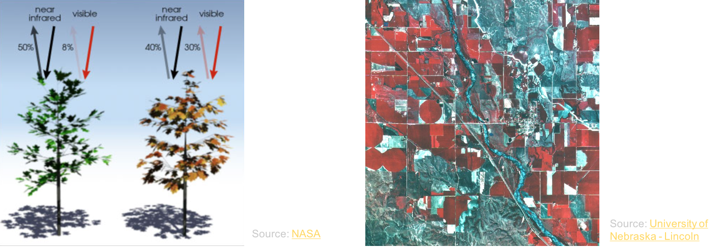
Gauging the health and productivity of plants throughout a growing season using their spectral signatures from imperfect satellite images is complex. To combat the many distortions of reflected light, such as the changing ratio of soil to plant canopy and the differing angles of the sun at the time of image creation, researchers have developed vegetation indices. A vegetation index is a formula relating the various wavelengths of light to plant canopy structures. Different indices are used to measure different qualities of cropland. For example, the Normalized Difference Vegetation Index (NDVI) that is a standard in agricultural remote sensing research and that is used in this project, is calculated using the red and near-infrared wavebands. It is applied to measure changes in the amount of green biomass over time, which can detect uneven patterns of growth. NDVI has also been used to solve other significant issues faced by those interested in measuring agricultural yields, including the identification and quantification of cropland 17 18, the tracking of field abandonment and recultivation 4, and the calculation of the intensity of cropland use 5.
Various vegetation indices have been used to predict crop yields. Comparisons of the performance of different indices are given in 6, 8, and 16. Indices are also combined with surface variables such as soil moisture, surface temperature, and rainfall to build more complex models (see 3 and 15).
Instead of adding more data to models predicting yields, this project has instead applied newer techniques in machine learning to pure vegetation index models. Other researchers have applied machine learning to agricultural remote sensing problems. Stepwise regression was used in 7 to predict rice production in China. Hierarchical clustering, Bayesian neural networks, and model-based recursive partitioning was used in 8 to predict barley, canola, and spring wheat yields on the Canadian Prairies. The authors in 9 trained a neural network using the shuffled complex evolution optimization algorithm developed at the University of Arizona (SCE-UA) to predict corn and soybean yields at the county level in the US corn belt. Random forests were used in 10 and 19 to classify pixels in satellite images into different categories of land uses. In 11, unsupervised linear unmixing was used on hyperspectral data to discriminate between soil and vegetation within one pixel. Multilayer perceptrons and radial basis functions were used in 13 to predict the crop area and yields of corn fields in India.
This project uses time series of satellite images across one growing cycle to predict soybean yields in Brazil. For some of our models, we turned these time series of NDVI values into trajectories and used them to predict yields at one point in time, as is done in 12. We also applied convolutional neural networks to our time series of satellite images in a way similar to this paper1.
If I have seen further it is by standing on the shoulders of giants.
- Sir Issac Newton
The Present - Users and Key Stakeholders
Defining the User
There are many constituents who can benefit from yield predictions for soybeans and other crops, including farmers, policy-makers, research houses and traders. For the purpose of this research project, the primary user was deemed to be the commodities traders who deal with buying and selling futures on a day-to-day basis. They are the individuals who help make the market (and as a result prices), and access to crop yield estimates has a direct impact on market dynamics.
Research Approach
In an effort to help guide our research, the team solicited feedback from a small group of commodities traders, which was collected through an online questionnaire. Because of the narrow audience, the data collection was limited to 5 respondents. However, the results provided good directional feedback that helped shape our research.
- Below are the list of questions asked, which were meant to allow for open ended responses:
- What types of financial instruments do you trade? If you trade commodities futures, which specific commodities?
- What type of data factors into your trading decision making?
- For commodities futures, have you ever used signals from non-traditional or relatively new data sources (i.e. something that you just started using in the past 2 years)? If so, please describe these new data sources.
- How important would it be to have accurate yield predictions as you assess commodities futures pricing (e.g. having an estimate for the corn yield for the harvest coming up in 6 months)?
- Do you have access to any sources of yield predictions today? How accurate are they?
- How much advance access to accurate yield predictions could give you a competitive advantage in pricing? (e.g. 1 year before harvest, 6 months before harvest, etc)
- At what resolution would you want yield predictions(nationwide yield estimates? county level? individual farms?)?
- Please add any other thoughts or comments that you think might be helpful as we work on this project.
Research Findings
- Generally, the respondents gave fairly consistent answers to most questions. The key takeaways that are most relevant to this project are listed in the bullets below:
- Some of the commonly used data sources cited by the respondents include: “fundamentals”, weekly statistics, market flows, macro themes and interest rates. These terms are broad and in some cases could include yield estimates.
- All respondents said that yield estimates would be important or very important to them. One respondent did indicate that yield estimates are available today, but typically closer to the harvest date.
- A subset of respondents had in-house research groups as well as external consultants who calculated yield estimates. However, there was interest in finding signals that may indicate if environmental changes may render the estimates obsolete.
- Having a longer time horizon for yield estimates is of great interest. However, there is a great degree of skepticism that estimates 1 year out will be accurate. In general, it appears that most accurate yield estimates occur 3 months prior to harvest.
- Most respondents felt that nationwide estimates would be the right level of granularity. One respondent saw value in county-level estimates.
Key Takeaways
- The research helped steer the project with the following guidelines:
- Focus on national predictions
- Include weather data, as this was deemed to be an important feature
- Primary value of this effort would be if a more accurate prediction could me made in a reasonably long time window (e.g. 3 - 6 months from harvest)
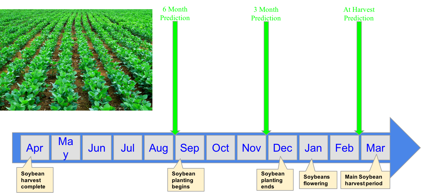
Brazillian Growth Cycle
I KEEP six honest serving-men
(They taught me all I knew);
Their names are What and Why and When
And How and Where and Who.
- The Elephant's Child, Sir Rudyard Kipling
Data Harvesting and Basic Wrangling
Farm Yield Data
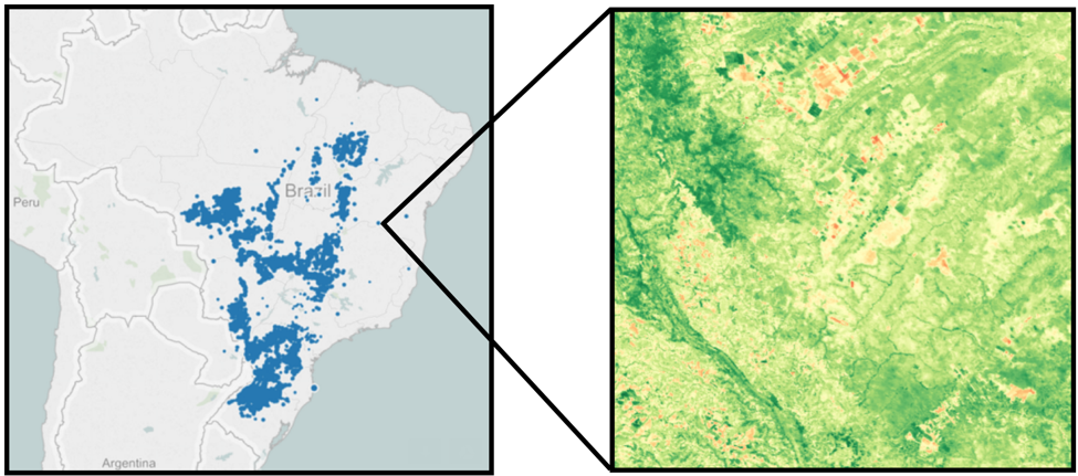
The farm-level soybean yield data we used was provided by a research team from Tufts University on special request. We express our gratitude to the team and to Prof. Coco Krumme for facilitating access to the data. The data contains fields such as dates, farm coordinates in latitude and longitude, yield calculation in metric tons per hectare, and many other agricultural indices for pestilence and disease (e.g. brown_stink_bug, cucurbit_beetle, fall_armyworm, false_medideira, green_stink_bug, snail, spodoptera_spp, stink_bug, tobacco_budworm, velvetbean_caterpillar and white_fly).
After removing all null data points, the visualization of the farm locations showed that we still had a very broad distribution over Brazil, necessitating a wide geographic area of satellite images in order to provide coverage over all the farms. Additionally, we noticed that some of the locations were outside of the geographic boundaries of Brazil. Further investigation showed that these locations had miscoded lat/long coordinates - either wrong sign of latitude and longitude, a zero value for one of the coordinates, or simply transposed latitude and longitude values. We chose to remove these data points to reduce any ambiguity regarding the validity of those farm locations.Satellite Data
Our primary data source was a subset of MODIS data, which provides Vegetation Indices every 16 days with a resolution of 250m. From the NASA website at http://modis.gsfc.nasa.gov/data/dataprod/mod13.php:
“MODIS (or Moderate Resolution Imaging Spectroradiometer) is a key instrument aboard the Terra(originally known as EOS AM-1) and Aqua (originally known as EOS PM-1) satellites. MODIS vegetation indices, produced on 16-day intervals and at multiple spatial resolutions, provide consistent spatial and temporal comparisons of vegetation canopy greenness, a composite property of leaf area, chlorophyll and canopy structure. Two vegetation indices are derived from atmospherically-corrected reflectance in the red, near-infrared, and blue wavebands; the normalized difference vegetation index (NDVI), which provides continuity with NOAA's AVHRR NDVI time series record for historical and climate applications, and the enhanced vegetation index (EVI), which minimizes canopy-soil variations and improves sensitivity over dense vegetation conditions. The two products more effectively characterize the global range of vegetation states and processes.”
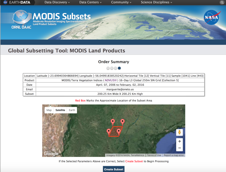 Due to stale MODIS product APIs and restrictions on download size per request, we could only manually download data as small grids in 200km by 200km sections. Considering the range of latitudes and longitudes of our farm locations, our initial calculations showed that we would have 165 different grids to download. However, further research narrowed that to only 64 grids (details below). The data collected is from April of 2006 to February of 2016, which contains 223 distinct satellite images in 16-day intervals. Only NDVI and EVI vegetation index files were downloaded, which was about 1GB each per grid per day and 128GB in total.
 At the outset, we noticed that the MODIS website only allows two parameters for data requests: the center coordinates and distance from the center. It then generates a square-like grid. It is important to note that it is not a perfect square because, as the latitude changes, delta distance per degree change in longitude on the globe also changes. Therefore, we cannot think in a 2-D world and simply calculate the grids by dividing longitude by some constant, because that will either result in extra grid count (due to too little unit longitude change each time), or uncovered area (due to too big unit longitude change each time). Instead, we used the max latitude and longitude as the starting point and calculated the coordinates of the next grid center by subtracting degree changes in latitude and longitude that resulted in 200km changes of spherical distance. We repeated this until we had covered the minimal value of latitudes and longitudes needed to include all of our farms.
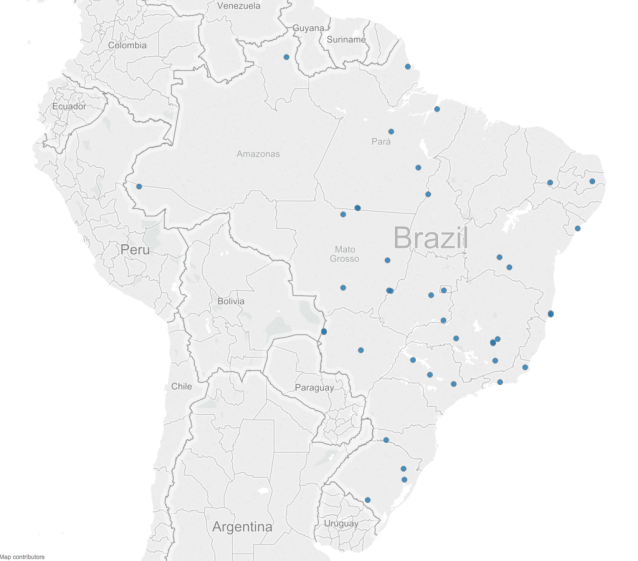
 We had a total of 165 grids that covered all our farm locations. However, not all of them had a farm in it. We then matched each farm to its nearest grid according to the farm-to-grid center distance. After this step, we realized that there were 82 grids that contained no farms and 19 grids that contained only 1 or 2 farms. Considering these farms do not exist in all years of yield data and their minimal effect on the total yield, we decide to filter them out, which resulted in only 64 grids for download. Each of the grids we downloaded contained at least 5 farms. After manually assigning thirteen grids to each of our teammates for download, we made our data requests at http://daacmodis.ornl.gov/cgi-bin/MODIS/GLBVIZ_1_Glb/modis_subset_order_global_col5.pl, and were notified via email once our data set was ready. The response time ranged from 40 minutes to 3 days.
Weather Data
Our initial weather data source was the NOAA repository. GHCND (Global Historical Climatology Network) maintains different summaries based on data exchanged under the World Meteorological Organization (WMO) World Weather Watch Program. Absent API access, we resorted to manual downloads of the monthly summaries from http://www.ncdc.noaa.gov/cdo-web/search.
 After investigation of the NOAA weather dataset on Brazil, it was found that our monthly summaries were very sparse, with about 50% of the data being NA values. We immediately started on a quest for alternative sources for this missing weather data and came upon Tutiempo. Tutiempo contains historical climate information for every country in the world. In the case of Brazil, it has data sets from more than 100 weather stations, and most of them contain the most recent 10 years of weather data that we needed. Since an API was not available, we programmed a customized webpage scraper. The scraper generated and scraped through all the Tutiempo Brazil dataset URLs, downloaded the necessary data, and organized it into csv-formatted files. This ingestable format was categorized by weather station latitude and longitude. Since the Tutiempo website robot was fairly adept at disconnecting us, the scraper was designed to be restarted from the last point of failure. Once the data download was complete, we were able to gather the following fields:
 T: Average Temperature (°C)
TM: Maximum temperature (°C)
Tm: Minimum temperature (°C)
SLP: Atmospheric pressure at sea level (hPa)
H: Average relative humidity (%)
PP: Total rainfall and / or snowmelt (mm)
VV: Average visibility (Km)
V: Average wind speed (Km/h)
VM: Maximum sustained wind speed (Km/h)
VG: Maximum speed of wind (Km/h)
RA: Indicator whether there was rain or drizzle (In the monthly average, the total days it rained)
SN: Indicator if it snowed (In the monthly average, the total days it snowed)
TS: Indicator if there was a thunderstorm (In the monthly average, the total days with thunderstorms)
FG: Indicator whether there was fog (In the monthly average, the total days with fog)
War is ninety percent information.
- Napoleon Bonaparte
The Future: Modelling
Baseline Features and Labels
The first pass of modeling was built on a baseline data set consists of 1 training example for every farm/year combination. In other words, a given farm will have a measure of its soybean yield for a given year, say 2012. That same farm will have a different yield in 2013, and that would be recorded as a separate training example. The primary features for any given training example is the NDVI value for the center pixel in the associated satellite images for that farm over a given time period. Satellite images were collected twice a month starting 10 months before the given year’s harvest. The target variable is the yield (in metric tons per hectare) for that farm for that given year. A list of the features and target variable is included below:
Table 1 - Initial Model Features - Single Pixel Values
![]()
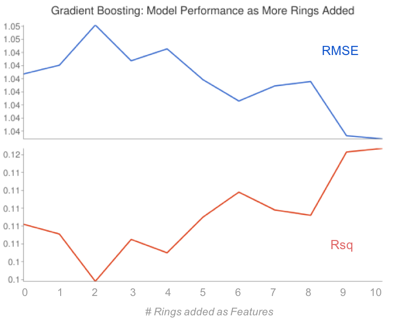
After running some initial models, it was decided to expand the area of pixels for which NDVI values were collected. Each pixel represents an area of 250m x 250m (about 15 acres), and without knowledge of the size of the farms, it seemed prudent to collect more than just the 1 pixel representing the centerpoint of the farm. Several “rings” of pixels were collected as is illustrated in Figure 1 below:
Figure 1 - Illustration of “Rings” as a parameter in feature engineering
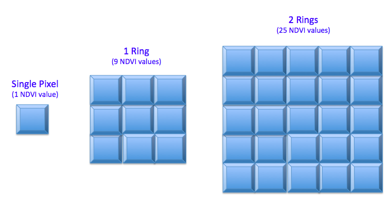
Table 2 - Model Features with n rings of pixels
As will be discussed later, expanding to 3 rings provided a material benefit to a simple OLS model. Based on this result, all further modeling efforts included at least 3 rings of NDVI data around the center pixel, and in many cases more.
Additional Data Cleaning & Training /Test Data Splits
 One issue that reduced the number of training examples were farms whose centers were close to an edge of the satellite image. For these farms, the rings of pixels were often truncated, resulting in only a partial data set. These examples were removed. Similarly, there were several N/A values. After trying various strategies to fill in missing values, including interpolation, it was shown that simply using the mean value of the satellite image was good enough.
The 7,456 remaining examples were split randomly into 5,964 training examples and 1,492 test examples. For this model, to keep the feature space small, 6 rings of pixel data were collected. However, an average of each ring was calculated, resulting in 7 pixel values (the center pixel value plus 6 averages) for each satellite image. Since there were 21 images per farm, the final feature space consisted of 147 pixel values (21 time periods x 7 pixel values per time
Incorporation of Weather Data
After spending some time with just the NDVI data, weather data was incorporated into the models as a new feature set. A summary of the related feature engineering is included below:
-
NOAA Weather Data:
- This data set had a lot of missing values. On average, each variable had more than 50% invalid values. Overall, only 1,755 observations out of 7,456 had complete weather data.
- Several variables were dropped that were mostly zero.
- Several variables that were heavily skewed were log transformed.
- The final training data set dimensions were 5,964 x 492 and the test set was 1,492 x 492.
- The large number of missing values and features resulted in very unstable models with negative R-squared values and large residuals.
-
Restructuring the Data Set:
- Instead of constructing the dataset with one farm per row, we reshaped it to be one image per row. This way, we have 21 times more rows and we could add image sequence as a dummy variable.
- New dimension of training set becomes 107,905 x 41, and testing set 26,977 x 41.
- Despite the missing values, the NOAA data added some predictive power to all models. We filled in the missing values with the variable mean.
-
Tutiempo Weather Data:
- Much better data quality. 101,667 out of 134,882 images had complete observations after dropping two mostly missing variables (VG and SLP).
- Log transformed FG, PP, RA, TS since they are right-skewed. Converted binary variable SN to a dummy variable.
- Final train set 81,333 x 54; final test set 20,334 x 54.
- Saw further improvements in results compared with NOAA.
-
Target variable transformation:
- Noticed that there were several very high yield farms that were really hard to predict.
- Log transformed the Yield variable and saw much better model performance.
Modeling Strategy & Metrics of Performance
Various classes of models were examined:
- Linear models (OLS)
- OLS
- Ridge Regression
- Non-linear models
- Support Vector Machines (SVM)
- Random Forest (RF)
- Gradient Boosting Decision Trees (GBDT)
- Neural Networks
- Convolutional (CNN) - http://danielnouri.org/notes/2014/12/17/using-convolutional-neural-nets-to-detect-facial-keypoints-tutorial/
- Recurrent (RNN) - http://www.wildml.com/2015/09/recurrent-neural-networks-tutorial-part-1-introduction-to-rnns/
- Gated Recurrent Units (GRU) - http://www.wildml.com/2015/10/recurrent-neural-network-tutorial-part-4-implementing-a-grulstm-rnn-with-python-and-theano/
Several metrics were used to compare performance across models:
Linear Models
- OLS
- Definition: Ordinary Least Squares regression models are the most basic form of linear regression models. An OLS model is built by finding parameters that minimize the squared distance between observed and predicted values of the dependent variable.
- Why we used them: We used OLS as a starting point to establish a simple baseline to which we could compare all additional models.
- What features were inputs: NDVI rings and weather data
- Ridge Regression
- Definition: Ridge regression is a variant of OLS regression where a regularization term is added to penalize parameter estimates which are large. This approach is often used to alleviate against multicollinearity.
- Why we used them: Given the nature of the data set (NDVI values in a time series), there was a risk of multicollinearity and, as a result, a high variance in parameter estimates. Therefore, we decided to use Ridge Regression as a follow on to OLS.
- What features were inputs: NDVI rings and weather data
Non-Linear Models
- Support Vector Regression (SVR)
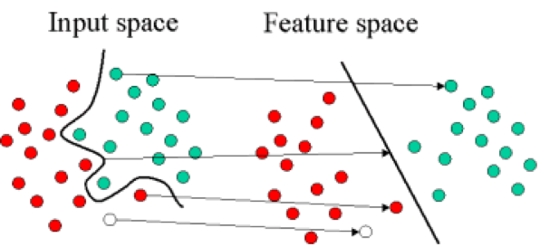
- Definition: Support Vector Regression uses Support Vector Machines (SVMs) to find a separating line/hyperplane that minimizes the distance between this plane and the yield values. In contrast to OLS, SVMs can produce non-linear 'best fit' curves. It does this by using non-linear kernels to transform the parameter space and working in this transformed space to find optimal linear support vectors. When these linear support vectors are transformed back into the original parameter space, they can become non-linear.
- Why we used them: We suspected that our yield prediction problem was non-linear.
- What features were inputs: NDVI rings and weather data
- Random Forest (RF)
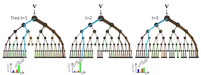
- Definition: Random forest models fall under a class of ensemble models that take collections of decision trees and use the mean prediction across the trees. Decision tree models are learning algorithms which have a decision flow structure. Each node asks a question about a feature, and the resulting branches represent “decisions” made based on the value of that feature.
- Why we used them: The initial linear models that we ran were found to have poor predictive power (initial R-squared values were in the range of 0.05 - 0.10). Given the complex nature of the dataset (e.g. time series of arrays of NDVI pixel values), it seemed logical to explore non-linear models. Random Forests are known to be the most generally robust across various classes of problems. For example, they are very good at handling outliers, of which there were many in this dataset.
- What features were inputs: NDVI rings and weather data
- Gradient Boosting Decision Trees (GBDT)
- Definition: This class of models is also an ensemble of decision trees. However, unlike Random Forests, GBDTs iteratively build new predictors from linear combinations of baseline weak learners (i.e. shallow trees that have high bias and low variance) using the gradient of the loss function as a key parameter.
- Why we used them: Since Random Forests use ensembles of fully grown trees, and therefore tend to have lower bias and higher variance, it seemed prudent to take an alternate approach with GBDTs which are iteratively built on weak learners that tend to be on the opposite end of the bias / variance tradeoff (weak learners with high bias and low variance).
- What features were inputs: NDVI rings and weather data
Results of Linear and Non-Linear Models
| Model | MSE | RMSE | MAE | MAPE | R-squared | Var Explained | Training Dim | Testing Dim | # Rings | Weather | Year Categ | Image Categ | Missing Pixel | Missing Weather |
|---|---|---|---|---|---|---|---|---|---|---|---|---|---|---|
| OLS | 0.0709 | 0.2664 | 0.2051 | 0.1962 | 0.1112 | 0.1113 | 81195x54 | 20299x54 | 10 | tutiempo | 1 | 1 | 0.5 | exclude |
| Ridge | 0.0709 | 0.2664 | 0.2051 | 0.1962 | 0.1113 | 0.1113 | 81195x54 | 20299x54 | 10 | tutiempo | 1 | 1 | 0.5 | exclude |
| SVR | 0.0640 | 0.2530 | 0.1956 | 0.1838 | 0.1984 | 0.1990 | 81195x54 | 20299x54 | 10 | tutiempo | 1 | 1 | 0.5 | exclude |
| RF | 0.0646 | 0.2542 | 0.1944 | 0.1762 | 0.1904 | 0.1905 | 81195x54 | 20299x54 | 10 | tutiempo | 1 | 1 | 0.5 | exclude |
| GB | 0.0653 | 0.2556 | 0.1982 | 0.1860 | 0.1814 | 0.1814 | 81195x54 | 20299x54 | 10 | tutiempo | 1 | 1 | 0.5 | exclude |
| OLS | 0.0700 | 0.2646 | 0.2036 | 0.1916 | 0.1061 | 0.1061 | 59528x48 | 14883x48 | 10 | tutiempo | 1 | 1 | 0.5 | exclude |
| Ridge | 0.0700 | 0.2646 | 0.2036 | 0.1916 | 0.1061 | 0.1061 | 59528x48 | 14883x48 | 10 | tutiempo | 1 | 1 | 0.5 | exclude |
| SVR | 0.0625 | 0.2499 | 0.1932 | 0.1794 | 0.2026 | 0.2033 | 59528x48 | 14883x48 | 10 | tutiempo | 1 | 1 | 0.5 | exclude |
| RF | 0.0614 | 0.2479 | 0.1891 | 0.1697 | 0.2157 | 0.2157 | 59528x48 | 14883x48 | 10 | tutiempo | 1 | 1 | 0.5 | exclude |
| GB | 0.0636 | 0.2522 | 0.1952 | 0.1804 | 0.1883 | 0.1883 | 59528x48 | 14883x48 | 10 | tutiempo | 1 | 1 | 0.5 | exclude |
| OLS | 0.0703 | 0.2652 | 0.2036 | 0.1945 | 0.1097 | 0.1099 | 40728x42 | 10182x42 | 10 | tutiempo | 1 | 1 | 0.5 | exclude |
| Ridge | 0.0703 | 0.2652 | 0.2036 | 0.1945 | 0.1098 | 0.1101 | 40728x42 | 10182x42 | 10 | tutiempo | 1 | 1 | 0.5 | exclude |
| SVR | 0.0635 | 0.2520 | 0.1952 | 0.1831 | 0.1965 | 0.1985 | 40728x42 | 10182x42 | 10 | tutiempo | 1 | 1 | 0.5 | exclude |
| RF | 0.0627 | 0.2504 | 0.1913 | 0.1745 | 0.2064 | 0.2067 | 40728x42 | 10182x42 | 10 | tutiempo | 1 | 1 | 0.5 | exclude |
| GB | 0.0638 | 0.2526 | 0.1958 | 0.1831 | 0.1926 | 0.1929 | 40728x42 | 10182x42 | 10 | tutiempo | 1 | 1 | 0.5 | exclude |
Neural Networks
Missing Values:
Missing values within a 13x13 image were replaced with the average value of the existing pixels in that image. Farms where there was one whole image of missing values (4,568 out of 9,162) were dropped from the analysis. This left 4,594 farms for training the models.
Feature Engineering:
The three types of neural networks we built required a different set of independent variables than the linear and nonlinear models discussed above. There were two main types of inputs to the models -- whole images and trajectories.
- Whole Images
- 1 image per farm: Time 20 (early February right before harvest)
- 7 images per farm: Time 14 - 20 (early November through early February - entire soybean growing season)
- Trajectories (Short Time Series)
- 1 trajectory of values through time for each pixel - 169 trajectories per farm
- Single Trajectory (7 values - early November through early February)
- Differences with 3 Lags (7 values - early November through early February and their lagged differences)
- Percent Differences with 3 Lags (7 values - early November through early February and their lagged percentage differences)
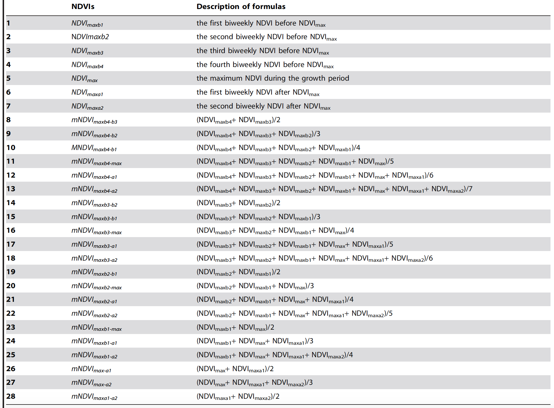
- From Maximum (10 Images Before, 2 Images After): Because we do not know when a field was planted, it is difficult to know on a particular date what stage of growth plants have reached. It is a standard assumption in remote sensing that the maximum NDVI value in a trajectory represents the peak of growth and greening for plants. For soybeans, this roughly means that harvest takes place two images, or four weeks, after maximum NDVI. It is therefore customary to find the maximum value and take the ten images before and the two images after it, giving a total trajectory length of 13 values.
- Averages from Maximum (similar to 7. See table below.)
- Differences from Maximum
- Percentage Differences from Maximum
- Single Trajectory from Maximum
Averages from Maximum:
From [7] Huang J, Wang X, Li X, Tian H, Pan Z (2013) Remotely Sensed Rice Yield Prediction Using Multi-Temporal NDVI Data Derived from NOAA's-AVHRR. PLoS ONE 8(8): e70816. doi:10.1371/journal.pone.0070816
- Convolutional Neural Networks (CNN)
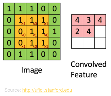
- Definition: Convolutional neural networks are modeled after the visual cortex in the human brain. When humans take in a visual image, the brain breaks it up into overlapping tiles. The neurons in the visual cortex then work over these tiles to detect patterns. CNNs take in an image of pixel values and similarly break it up into overlapping sub-images to detect patterns. This convolution happens at the beginning of the algorithm, before the perceptrons in the neural network do their job. Because the convolutions will pick up patterns that are then fed into the neurons, the user can do minimal preprocessing of the data. We built 5-layer CNNs, with 3 convolutional layers (that included subsampling and pooling) and two globally connected neural layers using Python’s Theano module.
- Why we used them: We are working with images, and this framework obviates the need for preprocessing.
- What features were inputs: Our first set of CNNs were fed whole images. The second set were fed trajectories.
- Code: Link to iPython Notebook
Model Target Value Features Data MAPE 1 5-layer with 1 channel yield Trajectories - from all 21 images/time periods - [1 x 21] array of NDVI values 13 Grids - 228,082 training examples Predictions were off by 45%. 2 3-layer with 1 channel yield Image at Time 20 (beginning of February, right before harvest) - [1 x 169] array of NDVI values 13 Grids - 1,180 training examples Predictions were off by 29%. 3 3-layer with 21 channels yield All 21 Images: Time0 to Time20 (early April through early Feburary) - [1 x 3549] array of NDVI values 13 Grids - 1,180 training examples Predictions were off by 26% 4 3-layer with 21 channels yield All 21 Images: Time0 to Time20 (early April through early Feburary) - [1 x 3549] array of NDVI values All 64 Grids - 7,127 training examples Predictions were off by 39%. 5 5-layer with 21 channels yield All 21 Images: Time0 to Time20 (early April through early Feburary) - [1 x 3549] array of NDVI values All 64 Grids - 7,127 training examples Predictions were off by 37%. 6 5-layer with 1 channel yield All 21 Images: Time0 to Time20 (early April through early Feburary) - [1 x 3549] array of NDVI values All 64 Grids - 7,127 training examples Predictions were off by 55%. 7 5-layer with 11 channels yield 11 Images: Time10 to Time20 (early September through early February) - [1 x 1859] array of NDVI values All 64 Grids - 7,127 training examples Predictions were off by 37%. 8 5-layer with 1 channel yield Trajectory Differences - 3 Lags - 11 Images (early September through early February) - [1 x 38] array of NDVI values All 64 Grids - 1,204,632 training examples Predictions were off by 74%. 9 5-layer with 1 channel yield Trajectory from Max NDVI Value - Averages - 7 images - [1 x 28] array of NDVI values All 64 Grids - 777,213 training examples Predictions were off by 49%. 10 5-layer with 1 channel yield Trajectory from Max NDVI Value - Differences - 3 Lags - 7 images - [1 x 22] array of NDVI values All 64 Grids - 777,213 training examples Predictions were off by 46%. 11 5-layer with 1 channel yield Replaced Missing Values - Trajectory from Max NDVI Value - Percentage Differences - 3 Lags - 7 images - [1 x 22] array of NDVI values All 64 Grids - 483,327 training examples Predictions were off by 54%. Image = 13x13 grid of pixels around each farm lat/lon = 169 total pixels
Trajectory = For one pixel, take the NDVI values across images/across time periods = 169 trajectories for each farm.
21 Images for each farm = early April of prior year to early February of current year.
Missing Values = 0.5
Note: Soybean growing season is November of previous year to February of current year. - Definition: Convolutional neural networks are modeled after the visual cortex in the human brain. When humans take in a visual image, the brain breaks it up into overlapping tiles. The neurons in the visual cortex then work over these tiles to detect patterns. CNNs take in an image of pixel values and similarly break it up into overlapping sub-images to detect patterns. This convolution happens at the beginning of the algorithm, before the perceptrons in the neural network do their job. Because the convolutions will pick up patterns that are then fed into the neurons, the user can do minimal preprocessing of the data. We built 5-layer CNNs, with 3 convolutional layers (that included subsampling and pooling) and two globally connected neural layers using Python’s Theano module.
- Recurrent Neural Networks (RNN)
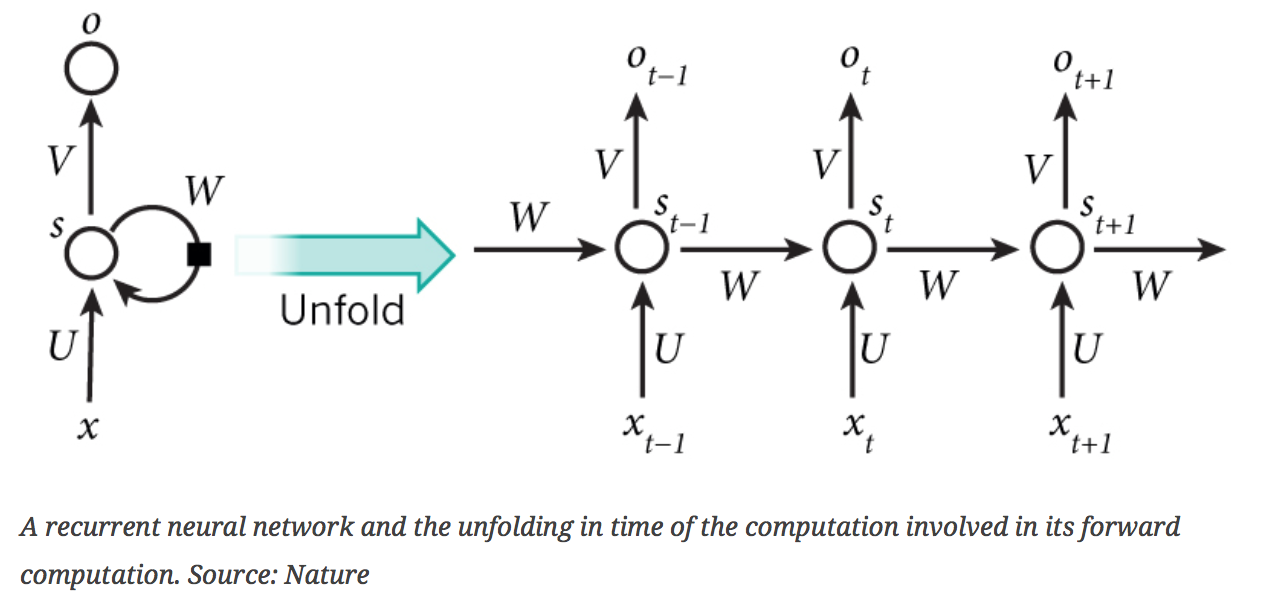
- Definition: Recurrent Neural Networks have memory. They take in a series of values collected over time (x) and predict an outcome at each time step (o). The prediction depends on the series of input values that came before it. Information from previous steps -- the memory (s) -- is encoded in a directed neural network. We built RNNs using Python’s Theano module.
- Why we used them: We wanted to take a sequence of NDVI values and make predictions of the yield all along the soybean growing cycle. We wanted to see how early we could start to make accurate predictions.
- What features were inputs: In our first set of models, we used trajectories only. In our second set of models, we used NDVI rings and weather data.
- Code: Link to iPython Notebook
Model Target Value Missing Values Epochs Features Data MAPE 1 tanh rectifier log(yield) Replaced with image average 100 Trajectory from Max NDVI Value - 4 before/2 after - 7 images - [1 x 7] array of NDVI values 10,000 training examples Predictions were off by 26%. 2 softplus rectifier yield Replaced with image average 100 Trajectory from Max NDVI Value - 4 before/2 after - 7 images - [1 x 7] array of NDVI values 64 Grids - 483,327 training examples Predictions were off by 40%. 3 softplus rectifier - 200 hidden nodes log(yield) Replaced with image average 1000 Trajectory from Max NDVI Value - 10 before/2 after - 13 images - 0 Rings - Tutiempo Weather Data 64 Grids - 1,934 training examples Predictions were off by 34%. 4 softplus rectifier - 500 hidden nodes log(yield) Replaced with image average 1000 Trajectory from Max NDVI Value - 10 before/2 after - 13 images - 10 Rings - Tutiempo Weather Data 64 Grids - 1,201 training examples Predictions were off by 52%. - Gated Recurrent Units (GRU)
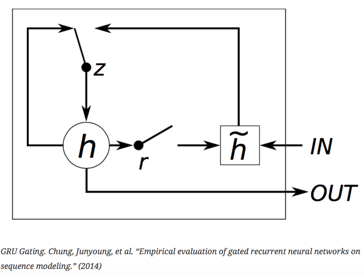
- Definition: Gated Recurrent Units are a generalization of RNNs. They also have memory, but their memory is dynamic. At each time step, gates are used to decide which new information to let in and which old information to let go. We built GRUs with two gated layers and an embedding layer using Python’s Theano module.
- Why we used them: GRUs allow longer sequences of information to be remembered.
- What features were inputs: We used trajectories only.
- Code: Link to iPython Notebook
Model Target Value Missing Values Epochs Features Data MAPE 1 2-layer log(yield) Replaced with image average 100 Trajectory from Max NDVI Value - 4 before/2 after - 7 images - [1 x 7] array of NDVI values 10,000 random training examples Predictions were off by 25%. 2 2-layer yield Replaced with image average 3 Trajectory from Max NDVI Value - 4 before/2 after - 7 images - [1 x 7] array of NDVI values 10,000 random training examples Predictions were off by 41%.
Conclusions
Our Goals
- The goals of this project were three-fold:
- Assess the predictive power of satellite images and weather data
- Compare and contrast modeling strategies
- Assess model accuracy as a function of time horizon
First, in our assessments, we found that satellite images are measurably effective inputs for predicting yields. The yield models become even more robust when weather data is added. This is important because this data is easily accessible, as compared to the data used in the most cutting-edge models. The USDA is the gold standard, and their models incorporate many measurements directly from the fields, which requires boots on the ground analyzing samples and interviewing farmers about their techniques.
Second, we found that the most effective models at predicting yields using satellite and weather data are Random Forests. In particular, our best-performing Random Forest models had ten trees and were trained using mean-squared error as the objective function. We also gave the trees maximum latitude by extending their limits to making splits with any node that had a minimum of two samples and creating leafs, or end nodes, that had at least one sample.
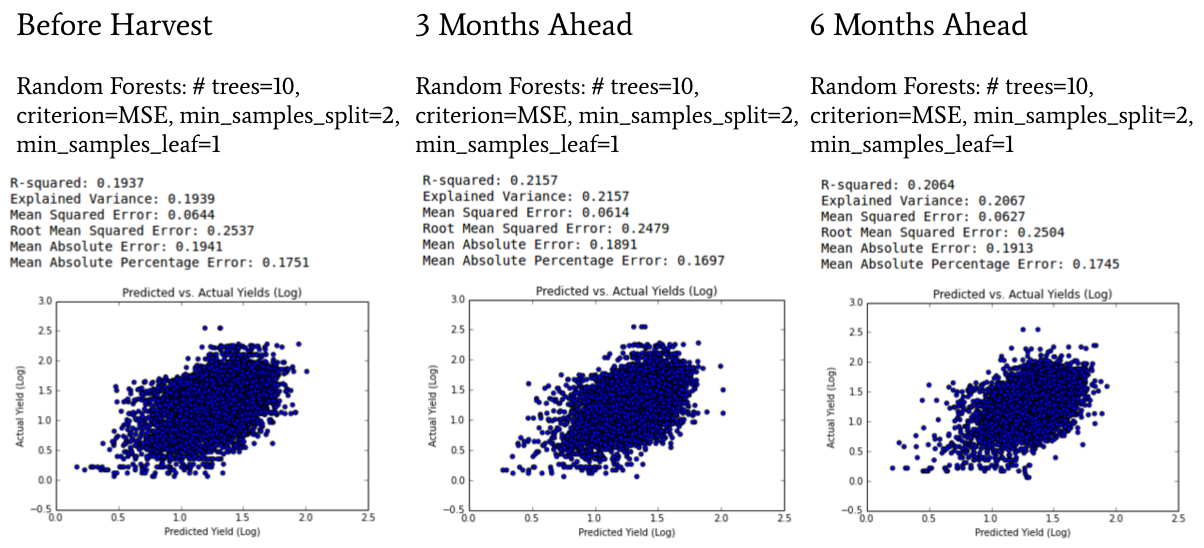
The results of our model comparisons are listed in the tables below. The first table shows how our models performed right before harvest, when they had all the data from the growing season as inputs. Both Support Vector Regression and Random Forests were effective in this timeframe. The second table shows how our models performed three months ahead of harvest. Here, Random Forest models are the clear winner. The third table shows how our models performed six months ahead of harvest. Again, Random Forests were the top performing model.
Before Harvest Model Results
| R-squared | RMSE | MAE | MAPE | |
|---|---|---|---|---|
| Baseline: Mean Model | 0.00% | 0.9664 | 0.7597 | 34.87% |
| OLS Regression | 11.12% | 0.2664 | 0.2051 | 19.62% |
| Ridge Regression | 11.13% | 0.2664 | 0.2051 | 19.62% |
| Support Vector Regression | 19.84% | 0.253 | 0.1956 | 18.38% |
| Random Forests | 19.04% | 0.2542 | 0.1944 | 17.62% |
| Gradient Boosting Decision Trees | 18.14% | 0.2556 | 0.1982 | 18.60% |
| Convolutional Neural Network | -4.98% | 0.9767 | 0.7533 | 24.63% |
| Recurrent Neural Network | 17.87% | 0.8776 | 0.6736 | 22.17% |
| Gated Recurrent Units | -1.62% | 0.9762 | 0.7596 | 25.28% |
Late Planting Season Model Results (3 months ahead)
| R-squared | RMSE | MAE | MAPE | |
|---|---|---|---|---|
| Baseline: Mean Model | 0.00% | 0.9664 | 0.7597 | 34.87% |
| OLS Regression | 10.61% | 0.2646 | 0.2036 | 19.16% |
| Ridge Regression | 10.61% | 0.2646 | 0.2036 | 19.16% |
| Support Vector Regression | 20.26% | 0.2499 | 0.1932 | 17.94% |
| Random Forests | 21.57% | 0.2479 | 0.1891 | 16.97% |
| Gradient Boosting Decision Trees | 18.83% | 0.2522 | 0.1952 | 18.04% |
| Convolutional Neural Network | NA | NA | NA | NA |
| Recurrent Neural Network | -9.03% | 1.0459 | 0.8051 | 32.18% |
| Gated Recurrent Units | -5.70% | 0.9956 | 0.7588 | 24.22% |
Early Planting Season Model Results (6 months ahead)
| R-squared | RMSE | MAE | MAPE | |
|---|---|---|---|---|
| Baseline: Mean Model | 0.00% | 0.9664 | 0.7597 | 34.87% |
| OLS Regression | 10.97% | 0.2652 | 0.2036 | 19.45% |
| Ridge Regression | 10.98% | 0.2652 | 0.2036 | 19.45% |
| Support Vector Regression | 19.65% | 0.252 | 0.1952 | 18.31% |
| Random Forests | 20.64% | 0.2504 | 0.1913 | 17.45% |
| Gradient Boosting Decision Trees | 19.26% | 0.2526 | 0.1958 | 18.31% |
| Convolutional Neural Network | NA | NA | NA | NA |
| Recurrent Neural Network | -16.35% | 1.0805 | 0.8366 | 32.09% |
| Gated Recurrent Units | NA | NA | NA | NA |
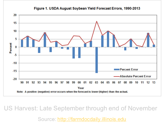
Finally, we found that our best predictions were made three months out from harvest. Our best model had a mean absolute percent error of 16.97%. When we compare our performance to that of the USDA’s more data-intensive models, we see that we did not outperform them, but we are getting closer. The graph below shows the USDA’s predictions three months out from harvest from 1990 through 2013. Their absolute percent error ranges from 1 to 16%. How much closer could we come to this gold standard with more research?
Future Research
- Ours is a rich dataset and is ripe for more model building and research. Here are some suggested next steps:
- First, to address the needs of our stakeholders, actual commodity prices should be incorporated into the models as targets and features. Unfortunately, we were not able to take our models that far due to employer compliance constraints.
- Second, our models look at very small subsets of satellite images to make predictions for one farm. The models should be adapted to take in regional and national level images to make predictions for these larger areas.
- Third, the Recurrent Neural Networks and Gated Recurrent Units could use more exploration. But in order to do this, the models need to run faster. The current code is by no means optimized and can use more development.
- Fourth, we have not incorporated the weather data into the RNN and GRU models. We believe this could significantly increase the performance of these models.
- Finally, we suggest testing alternative vegetation indices. We looked at NDVI and EVI. Others could be calculated, and models could be built using multiple indices as features. We never combined NDVI and EVI in the same model. This should be tried.
Zeus, whose will has marked for man
The sole way where wisdom lies;
Ordered one eternal plan:
Man must suffer to be wise.
- Agamemnon, by Aeschylus
Questions and Comments?
We welcome your questions and comments! Please use the form below to send us a quick note with your thoughts.
Additional data
Detailed Results of Linear and Non-Linear Models
| # Rings | Log Yield | Weather | Year Categ | Image Categ | Model | MSE | RMSE | R-squared | Var Explained | Training Dim | Testing Dim | Missing Pixel | Missing Weather | MAE | MAPE |
|---|---|---|---|---|---|---|---|---|---|---|---|---|---|---|---|
| One Farm Per Row | |||||||||||||||
| 0 | 0 | 0 | 0 | 0 | LR | 1.1761 | 1.0845 | 0.0366 | 0.0369 | 5964x21 | 1492x21 | 0.5 | NA | ||
| 0 | 0 | 0 | 0 | 0 | Ridge | 1.1758 | 1.0843 | 0.0368 | 0.0371 | 5964x21 | 1492x21 | 0.5 | NA | ||
| 0 | 0 | 0 | 0 | 0 | SVM | 1.1730 | 1.0831 | 0.0391 | 0.0412 | 5964x21 | 1492x21 | 0.5 | NA | ||
| 0 | 0 | 0 | 0 | 0 | RF | 1.2621 | 1.1234 | -0.0339 | -0.0339 | 5964x21 | 1492x21 | 0.5 | NA | ||
| 0 | 0 | 0 | 0 | 0 | GB | 1.1499 | 1.0723 | 0.0580 | 0.0581 | 5964x21 | 1492x21 | 0.5 | NA | ||
| 0 | 0 | 0 | 1 | 0 | LR | 1.1254 | 1.0608 | 0.0781 | 0.0783 | 5964x30 | 1492x30 | 0.5 | NA | ||
| 0 | 0 | 0 | 1 | 0 | Ridge | 1.1251 | 1.0607 | 0.0783 | 0.0785 | 5964x30 | 1492x30 | 0.5 | NA | ||
| 0 | 0 | 0 | 1 | 0 | SVM | 1.1302 | 1.0631 | 0.0741 | 0.0768 | 5964x30 | 1492x30 | 0.5 | NA | ||
| 0 | 0 | 0 | 1 | 0 | RF | 1.1671 | 1.0803 | 0.0440 | 0.0440 | 5964x30 | 1492x30 | 0.5 | NA | ||
| 0 | 0 | 0 | 1 | 0 | GB | 1.0886 | 1.0434 | 0.1082 | 0.1083 | 5964x30 | 1492x30 | 0.5 | NA | ||
| 1 | 0 | 0 | 1 | 0 | LR | 1.1274 | 1.0618 | 0.0764 | 0.0766 | 5964x51 | 1492x51 | 0.5 | NA | ||
| 1 | 0 | 0 | 1 | 0 | Ridge | 1.1264 | 1.0613 | 0.0772 | 0.0774 | 5964x51 | 1492x51 | 0.5 | NA | ||
| 1 | 0 | 0 | 1 | 0 | SVM | 1.1314 | 1.0637 | 0.0732 | 0.0762 | 5964x51 | 1492x51 | 0.5 | NA | ||
| 1 | 0 | 0 | 1 | 0 | RF | 1.1939 | 1.0927 | 0.0219 | 0.0220 | 5964x51 | 1492x51 | 0.5 | NA | ||
| 1 | 0 | 0 | 1 | 0 | GB | 1.0900 | 1.0440 | 0.1071 | 0.1072 | 5964x51 | 1492x51 | 0.5 | NA | ||
| 2 | 0 | 0 | 1 | 0 | LR | 1.1311 | 1.0635 | 0.0734 | 0.0735 | 5964x72 | 1492x72 | 0.5 | NA | ||
| 2 | 0 | 0 | 1 | 0 | Ridge | 1.1279 | 1.0620 | 0.0760 | 0.0762 | 5964x72 | 1492x72 | 0.5 | NA | ||
| 2 | 0 | 0 | 1 | 0 | SVM | 1.1294 | 1.0627 | 0.0748 | 0.0775 | 5964x72 | 1492x72 | 0.5 | NA | ||
| 2 | 0 | 0 | 1 | 0 | RF | 1.1699 | 1.0816 | 0.0416 | 0.0416 | 5964x72 | 1492x72 | 0.5 | NA | ||
| 2 | 0 | 0 | 1 | 0 | GB | 1.0964 | 1.0471 | 0.1018 | 0.1019 | 5964x72 | 1492x72 | 0.5 | NA | ||
| 3 | 0 | 0 | 1 | 0 | LR | 1.1368 | 1.0662 | 0.0688 | 0.0690 | 5964x93 | 1492x93 | 0.5 | NA | ||
| 3 | 0 | 0 | 1 | 0 | Ridge | 1.1299 | 1.0630 | 0.0744 | 0.0746 | 5964x93 | 1492x93 | 0.5 | NA | ||
| 3 | 0 | 0 | 1 | 0 | SVM | 1.1281 | 1.0621 | 0.0759 | 0.0784 | 5964x93 | 1492x93 | 0.5 | NA | ||
| 3 | 0 | 0 | 1 | 0 | RF | 1.1290 | 1.0625 | 0.0751 | 0.0753 | 5964x93 | 1492x93 | 0.5 | NA | ||
| 3 | 0 | 0 | 1 | 0 | GB | 1.0907 | 1.0444 | 0.1065 | 0.1066 | 5964x93 | 1492x93 | 0.5 | NA | ||
| 4 | 0 | 0 | 1 | 0 | LR | 1.1389 | 1.0672 | 0.0670 | 0.0671 | 5964x114 | 1492x114 | 0.5 | NA | ||
| 4 | 0 | 0 | 1 | 0 | Ridge | 1.1295 | 1.0628 | 0.0747 | 0.0749 | 5964x114 | 1492x114 | 0.5 | NA | ||
| 4 | 0 | 0 | 1 | 0 | SVM | 1.1261 | 1.0612 | 0.0775 | 0.0799 | 5964x114 | 1492x114 | 0.5 | NA | ||
| 4 | 0 | 0 | 1 | 0 | RF | 1.1641 | 1.0789 | 0.0464 | 0.0464 | 5964x114 | 1492x114 | 0.5 | NA | ||
| 4 | 0 | 0 | 1 | 0 | GB | 1.0926 | 1.0453 | 0.1050 | 0.1051 | 5964x114 | 1492x114 | 0.5 | NA | ||
| 5 | 0 | 0 | 1 | 0 | LR | 1.1433 | 1.0693 | 0.0634 | 0.0635 | 5964x135 | 1492x135 | 0.5 | NA | ||
| 5 | 0 | 0 | 1 | 0 | Ridge | 1.1300 | 1.0630 | 0.0743 | 0.0744 | 5964x135 | 1492x135 | 0.5 | NA | ||
| 5 | 0 | 0 | 1 | 0 | SVM | 1.1251 | 1.0607 | 0.0783 | 0.0808 | 5964x135 | 1492x135 | 0.5 | NA | ||
| 5 | 0 | 0 | 1 | 0 | RF | 1.1488 | 1.0718 | 0.0589 | 0.0589 | 5964x135 | 1492x135 | 0.5 | NA | ||
| 5 | 0 | 0 | 1 | 0 | GB | 1.0877 | 1.0429 | 0.1090 | 0.1091 | 5964x135 | 1492x135 | 0.5 | NA | ||
| 6 | 0 | 0 | 1 | 0 | LR | 1.1447 | 1.0699 | 0.0622 | 0.0623 | 5964x156 | 1492x156 | 0.5 | NA | ||
| 6 | 0 | 0 | 1 | 0 | Ridge | 1.1297 | 1.0629 | 0.0746 | 0.0747 | 5964x156 | 1492x156 | 0.5 | NA | ||
| 6 | 0 | 0 | 1 | 0 | SVM | 1.1246 | 1.0605 | 0.0788 | 0.0812 | 5964x156 | 1492x156 | 0.5 | NA | ||
| 6 | 0 | 0 | 1 | 0 | RF | 1.1674 | 1.0805 | 0.0437 | 0.0440 | 5964x156 | 1492x156 | 0.5 | NA | ||
| 6 | 0 | 0 | 1 | 0 | GB | 1.0843 | 1.0413 | 0.1118 | 0.1120 | 5964x156 | 1492x156 | 0.5 | NA | ||
| 7 | 0 | 0 | 1 | 0 | LR | 1.1431 | 1.0692 | 0.0636 | 0.0636 | 5964x177 | 1492x177 | 0.5 | NA | ||
| 7 | 0 | 0 | 1 | 0 | Ridge | 1.1266 | 1.0614 | 0.0771 | 0.0772 | 5964x177 | 1492x177 | 0.5 | NA | ||
| 7 | 0 | 0 | 1 | 0 | SVM | 1.1234 | 1.0599 | 0.0797 | 0.0821 | 5964x177 | 1492x177 | 0.5 | NA | ||
| 7 | 0 | 0 | 1 | 0 | RF | 1.1454 | 1.0702 | 0.0617 | 0.0619 | 5964x177 | 1492x177 | 0.5 | NA | ||
| 7 | 0 | 0 | 1 | 0 | GB | 1.0867 | 1.0424 | 0.1098 | 0.1100 | 5964x177 | 1492x177 | 0.5 | NA | ||
| 8 | 0 | 0 | 1 | 0 | LR | 1.1494 | 1.0721 | 0.0584 | 0.0585 | 5964x198 | 1492x198 | 0.5 | NA | ||
| 8 | 0 | 0 | 1 | 0 | Ridge | 1.1268 | 1.0615 | 0.0769 | 0.0770 | 5964x198 | 1492x198 | 0.5 | NA | ||
| 8 | 0 | 0 | 1 | 0 | SVM | 1.1224 | 1.0594 | 0.0805 | 0.0828 | 5964x198 | 1492x198 | 0.5 | NA | ||
| 8 | 0 | 0 | 1 | 0 | RF | 1.1449 | 1.0700 | 0.0621 | 0.0624 | 5964x198 | 1492x198 | 0.5 | NA | ||
| 8 | 0 | 0 | 1 | 0 | GB | 1.0874 | 1.0428 | 0.1092 | 0.1095 | 5964x198 | 1492x198 | 0.5 | NA | ||
| 9 | 0 | 0 | 1 | 0 | LR | 1.1557 | 1.0750 | 0.0532 | 0.0533 | 5964x219 | 1492x219 | 0.5 | NA | ||
| 9 | 0 | 0 | 1 | 0 | Ridge | 1.1273 | 1.0617 | 0.0765 | 0.0766 | 5964x219 | 1492x219 | 0.5 | NA | ||
| 9 | 0 | 0 | 1 | 0 | SVM | 1.1217 | 1.0591 | 0.0811 | 0.0834 | 5964x219 | 1492x219 | 0.5 | NA | ||
| 9 | 0 | 0 | 1 | 0 | RF | 1.1266 | 1.0614 | 0.0771 | 0.0773 | 5964x219 | 1492x219 | 0.5 | NA | ||
| 9 | 0 | 0 | 1 | 0 | GB | 1.0788 | 1.0387 | 0.1163 | 0.1164 | 5964x219 | 1492x219 | 0.5 | NA | ||
| 10 | 0 | 0 | 1 | 0 | LR | 1.1599 | 1.0770 | 0.0498 | 0.0498 | 5964x240 | 1492x240 | 0.5 | NA | ||
| 10 | 0 | 0 | 1 | 0 | Ridge | 1.1316 | 1.0638 | 0.0730 | 0.0731 | 5964x240 | 1492x240 | 0.5 | NA | ||
| 10 | 0 | 0 | 1 | 0 | SVM | 1.1211 | 1.0588 | 0.0816 | 0.0838 | 5964x240 | 1492x240 | 0.5 | NA | ||
| 10 | 0 | 0 | 1 | 0 | RF | 1.1261 | 1.0612 | 0.0775 | 0.0776 | 5964x240 | 1492x240 | 0.5 | NA | ||
| 10 | 0 | 0 | 1 | 0 | GB | 1.0783 | 1.0384 | 0.1167 | 0.1169 | 5964x240 | 1492x240 | 0.5 | NA | ||
| One Image Per Row | |||||||||||||||
| 10 | 0 | 0 | 0 | 0 | LR | 1.1543 | 1.0744 | 0.0010 | 0.0011 | 107905x11 | 26977x11 | 0.5 | NA | ||
| 10 | 0 | 0 | 0 | 0 | Ridge | 1.1543 | 1.0744 | 0.0010 | 0.0011 | 107905x11 | 26977x11 | 0.5 | NA | ||
| 10 | 0 | 0 | 0 | 0 | SVM | 1.1497 | 1.0722 | 0.0050 | 0.0060 | 107905x11 | 26977x11 | 0.5 | NA | ||
| 10 | 0 | 0 | 0 | 0 | RF | 1.2521 | 1.1190 | -0.0836 | -0.0836 | 107905x11 | 26977x11 | 0.5 | NA | ||
| 10 | 0 | 0 | 0 | 0 | GB | 1.1467 | 1.0708 | 0.0076 | 0.0077 | 107905x11 | 26977x11 | 0.5 | NA | ||
| 10 | 0 | 0 | 1 | 0 | LR | 1.0842 | 1.0412 | 0.0617 | 0.0618 | 107905x20 | 26977x20 | 0.5 | NA | ||
| 10 | 0 | 0 | 1 | 0 | Ridge | 1.0842 | 1.0412 | 0.0617 | 0.0618 | 107905x20 | 26977x20 | 0.5 | NA | ||
| 10 | 0 | 0 | 1 | 0 | SVM | 1.0838 | 1.0411 | 0.0620 | 0.0635 | 107905x20 | 26977x20 | 0.5 | NA | ||
| 10 | 0 | 0 | 1 | 0 | RF | 1.1480 | 1.0714 | 0.0065 | 0.0065 | 107905x20 | 26977x20 | 0.5 | NA | ||
| 10 | 0 | 0 | 1 | 0 | GB | 1.0755 | 1.0371 | 0.0692 | 0.0693 | 107905x20 | 26977x20 | 0.5 | NA | ||
| 10 | 0 | 0 | 1 | 1 | LR | 1.0845 | 1.0414 | 0.0614 | 0.0615 | 107905x41 | 26977x41 | 0.5 | NA | ||
| 10 | 0 | 0 | 1 | 1 | Ridge | 1.0845 | 1.0414 | 0.0615 | 0.0616 | 107905x41 | 26977x41 | 0.5 | NA | ||
| 10 | 0 | 0 | 1 | 1 | SVM | 1.0812 | 1.0398 | 0.0643 | 0.0659 | 107905x41 | 26977x41 | 0.5 | NA | ||
| 10 | 0 | 0 | 1 | 1 | RF | 1.1297 | 1.0629 | 0.0223 | 0.0223 | 107905x41 | 26977x41 | 0.5 | NA | ||
| 10 | 0 | 0 | 1 | 1 | GB | 1.0739 | 1.0363 | 0.0706 | 0.0707 | 107905x41 | 26977x41 | 0.5 | NA | ||
| 10 | 0 | NOAA | 1 | 1 | LR | 1.0455 | 1.0225 | 0.0952 | 0.0953 | 107905x41 | 26977x41 | 0.5 | fill in avg | ||
| 10 | 0 | NOAA | 1 | 1 | Ridge | 1.0455 | 1.0225 | 0.0952 | 0.0953 | 107905x41 | 26977x41 | 0.5 | fill in avg | ||
| 10 | 0 | NOAA | 1 | 1 | SVM | 0.9684 | 0.9841 | 0.1619 | 0.1663 | 107905x41 | 26977x41 | 0.5 | fill in avg | ||
| 10 | 0 | NOAA | 1 | 1 | RF | 1.0197 | 1.0098 | 0.1175 | 0.1175 | 107905x41 | 26977x41 | 0.5 | fill in avg | ||
| 10 | 0 | NOAA | 1 | 1 | GB | 0.9747 | 0.9873 | 0.1565 | 0.1565 | 107905x41 | 26977x41 | 0.5 | fill in avg | ||
| 10 | 0 | tutiempo | 1 | 1 | LR | 1.0286 | 1.0142 | 0.0872 | 0.0872 | 95152x53 | 23789x53 | 0.5 | exclude | ||
| 10 | 0 | tutiempo | 1 | 1 | Ridge | 1.0286 | 1.0142 | 0.0872 | 0.0872 | 95152x53 | 23789x53 | 0.5 | exclude | ||
| 10 | 0 | tutiempo | 1 | 1 | SVM | 0.9507 | 0.9750 | 0.1564 | 0.1594 | 95152x53 | 23789x53 | 0.5 | exclude | ||
| 10 | 0 | tutiempo | 1 | 1 | RF | 0.9411 | 0.9701 | 0.1649 | 0.1652 | 95152x53 | 23789x53 | 0.5 | exclude | ||
| 10 | 0 | tutiempo | 1 | 1 | GB | 0.9622 | 0.9809 | 0.1462 | 0.1462 | 95152x53 | 23789x53 | 0.5 | exclude | ||
| 10 | 0 | tutiempo | 1 | 1 | LR | 1.0479 | 1.0237 | 0.0855 | 0.0855 | 125260x53 | 31316x53 | 0.5 | fill in avg | ||
| 10 | 0 | tutiempo | 1 | 1 | Ridge | 1.0478 | 1.0236 | 0.0855 | 0.0855 | 125260x53 | 31316x53 | 0.5 | fill in avg | ||
| 10 | 0 | tutiempo | 1 | 1 | SVM | 0.9721 | 0.9860 | 0.1516 | 0.1541 | 125260x53 | 31316x53 | 0.5 | fill in avg | ||
| 10 | 0 | tutiempo | 1 | 1 | RF | 0.9555 | 0.9775 | 0.1661 | 0.1661 | 125260x53 | 31316x53 | 0.5 | fill in avg | ||
| 10 | 0 | tutiempo | 1 | 1 | GB | 0.9893 | 0.9946 | 0.1366 | 0.1366 | 125260x53 | 31316x53 | 0.5 | fill in avg | ||
| 10 | 0 | tutiempo, cate_SN | 1 | 1 | LR | 1.0715 | 1.0351 | 0.0882 | 0.0883 | 81333x54 | 20334x54 | linear interpolate | exclude | ||
| 10 | 0 | tutiempo, cate_SN | 1 | 1 | Ridge | 1.0715 | 1.0351 | 0.0882 | 0.0883 | 81333x54 | 20334x54 | linear interpolate | exclude | ||
| 10 | 0 | tutiempo, cate_SN | 1 | 1 | SVM | 0.9988 | 0.9994 | 0.1501 | 0.1531 | 81333x54 | 20334x54 | linear interpolate | exclude | ||
| 10 | 0 | tutiempo, cate_SN | 1 | 1 | RF | 1.0300 | 1.0149 | 0.1235 | 0.1238 | 81333x54 | 20334x54 | linear interpolate | exclude | ||
| 10 | 0 | tutiempo, cate_SN | 1 | 1 | GB | 1.0042 | 1.0021 | 0.1455 | 0.1456 | 81333x54 | 20334x54 | linear interpolate | exclude | ||
| Log Transformation on Yield: All measurements are in Log Term (Removed Yield=0) | |||||||||||||||
| 10 | 1 | tutiempo, cate_SN | 1 | 1 | LR | 0.0709 | 0.2664 | 0.1112 | 0.1113 | 81195x54 | 20299x54 | 0.5 | exclude | 0.2051 | 0.1962 |
| 10 | 1 | tutiempo, cate_SN | 1 | 1 | Ridge | 0.0709 | 0.2664 | 0.1113 | 0.1113 | 81195x54 | 20299x54 | 0.5 | exclude | 0.2051 | 0.1962 |
| 10 | 1 | tutiempo, cate_SN | 1 | 1 | SVM | 0.0640 | 0.2530 | 0.1984 | 0.1990 | 81195x54 | 20299x54 | 0.5 | exclude | 0.1956 | 0.1838 |
| 10 | 1 | tutiempo, cate_SN | 1 | 1 | RF | 0.0646 | 0.2542 | 0.1904 | 0.1905 | 81195x54 | 20299x54 | 0.5 | exclude | 0.1944 | 0.1762 |
| 10 | 1 | tutiempo, cate_SN | 1 | 1 | GB | 0.0653 | 0.2556 | 0.1814 | 0.1814 | 81195x54 | 20299x54 | 0.5 | exclude | 0.1982 | 0.1860 |
| 10 | 1 | tutiempo, cate_SN | 0 | 1 | LR | 0.0775 | 0.2784 | 0.0565 | 0.0566 | 81333x45 | 20334x45 | 0.5 | exclude | 0.2102 | 0.2019 |
| 10 | 1 | tutiempo, cate_SN | 0 | 1 | Ridge | 0.0775 | 0.2784 | 0.0566 | 0.0566 | 81333x45 | 20334x45 | 0.5 | exclude | 0.2102 | 0.2019 |
| 10 | 1 | tutiempo, cate_SN | 0 | 1 | SVM | 0.0659 | 0.2567 | 0.1971 | 0.1989 | 81333x45 | 20334x45 | 0.5 | exclude | 0.1970 | 0.1836 |
| 10 | 1 | tutiempo, cate_SN | 0 | 1 | RF | 0.0680 | 0.2608 | 0.1723 | 0.1723 | 81333x45 | 20334x45 | 0.5 | exclude | 0.1986 | 0.1775 |
| 10 | 1 | tutiempo, cate_SN | 0 | 1 | GB | 0.0692 | 0.2631 | 0.1576 | 0.1576 | 81333x45 | 20334x45 | 0.5 | exclude | 0.2018 | 0.1887 |
| Three Month Ahead Prediction: log Transformation on Yield, Removed Yield=0 | |||||||||||||||
| 10 | 1 | tutiempo, cate_SN | 1 | 1 | LR | 0.0700 | 0.2646 | 0.1061 | 0.1061 | 59528x48 | 14883x48 | 0.5 | exclude | 0.2036 | 0.1916 |
| 10 | 1 | tutiempo, cate_SN | 1 | 1 | Ridge | 0.0700 | 0.2646 | 0.1061 | 0.1061 | 59528x48 | 14883x48 | 0.5 | exclude | 0.2036 | 0.1916 |
| 10 | 1 | tutiempo, cate_SN | 1 | 1 | SVM | 0.0625 | 0.2499 | 0.2026 | 0.2033 | 59528x48 | 14883x48 | 0.5 | exclude | 0.1932 | 0.1794 |
| 10 | 1 | tutiempo, cate_SN | 1 | 1 | RF | 0.0614 | 0.2479 | 0.2157 | 0.2157 | 59528x48 | 14883x48 | 0.5 | exclude | 0.1891 | 0.1697 |
| 10 | 1 | tutiempo, cate_SN | 1 | 1 | GB | 0.0636 | 0.2522 | 0.1883 | 0.1883 | 59528x48 | 14883x48 | 0.5 | exclude | 0.1952 | 0.1804 |
| Six Month Ahead Prediction: log Transformation on Yield, Removed Yield=0 | |||||||||||||||
| 10 | 1 | tutiempo, cate_SN | 1 | 1 | LR | 0.0703 | 0.2652 | 0.1097 | 0.1099 | 40728x42 | 10182x42 | 0.5 | exclude | 0.2036 | 0.1945 |
| 10 | 1 | tutiempo, cate_SN | 1 | 1 | Ridge | 0.0703 | 0.2652 | 0.1098 | 0.1101 | 40728x42 | 10182x42 | 0.5 | exclude | 0.2036 | 0.1945 |
| 10 | 1 | tutiempo, cate_SN | 1 | 1 | SVM | 0.0635 | 0.2520 | 0.1965 | 0.1985 | 40728x42 | 10182x42 | 0.5 | exclude | 0.1952 | 0.1831 |
| 10 | 1 | tutiempo, cate_SN | 1 | 1 | RF | 0.0627 | 0.2504 | 0.2064 | 0.2067 | 40728x42 | 10182x42 | 0.5 | exclude | 0.1913 | 0.1745 |
| 10 | 1 | tutiempo, cate_SN | 1 | 1 | GB | 0.0638 | 0.2526 | 0.1926 | 0.1929 | 40728x42 | 10182x42 | 0.5 | exclude | 0.1958 | 0.1831 |